Building an ETL pipeline on Google Cloud

When was the last time you booked accommodation without checking its photos? Most probably never! Because having imagery information makes our decision-making process much easier and faster. However, picking up the best possible images of a hotel to show to the user is an interesting problem to solve, because it can be a naive random selection or a sophisticated machine learning model to know what the user truly wants at that moment.

This is why we at trivago have a dedicated Extract-Transform-Load (ETL) pipeline to create the image galleries for accommodations. This pipeline will generate a sorted image gallery for a given accommodation considering several parameters such as content on the image (represented by the image tag) and the quality of the image.

We initially had this pipeline on Amazon Web Services (AWS) and we recently migrated it to run on Google Cloud Platform (GCP). We did a complete redesign of the architecture when we migrated, not just because they are two different cloud platforms, but also because we wanted to add more features and stability to the pipeline.

However, no software project is a smooth ride, and we’re going to talk about the problems we faced and how we tried to fix most of them.

Architecture

The GCP service we use mostly for this pipeline is Dataflow: a fully managed service for Apache Beam pipelines. It gives us a lot of flexibility in logically separating each step of our process in generating the image galleries. We have separate Dataflow jobs performing different tasks including generating the galleries, validating the galleries, and finally streaming the galleries using a Kafka topic to the frontend teams.

Key Components:

• Images Snapshooter
  Generates the Images snapshot of all the active images.
• Tags Snapshooter
  Generates the Image Tags snapshot with the tags for the images.
• Changed Accommodations Fetcher
  Extracts the changed accommodations (using the changed images).
• Gallery Builder
  Builds the image galleries with the corresponding sorting order for the images and the updates for the changed accommodations.
• Gallery Snapshooter
  Creates the Image Gallery snapshot.
• Validator
  Validates the snapshot to ensure the images are in the correct order.
• Streamer
  Streams the changes if the validation step is passed.
• Orchestrator
  Orchestrates the different Dataflow jobs one after the other.

Terminology

• Data Lake
  A shared GCP account that is used by different teams in order to exchange their outputs with other teams.
• Snapshot State of a dataset at a given point in time. This can also be considered as a backup of the data at that time.

Challenges

Creating this kind of a complex pipeline doesn’t come easy, but with a lot of orchestration and edge cases to take into account.

Passing dynamic parameters

These Dataflow jobs need to be run daily in sequence with corresponding parameters denoting the input and output locations. These parameters change over the runs and the classic Dataflow templates don’t allow us to pass dynamic parameters to a Dataflow job. So, we moved all our Dataflow jobs to use Flex templates and it’s way easier to deploy because they use Docker images stored in Google Container Registry (GCR) to host our code and its dependencies.

With Flex templates, the Directed Acyclic Graph (DAG) for the Apache Beam pipeline is generated during the runtime depending on the parameters we pass and this allows us to make our code more modular and testable.

To read more about how to use Flex templates, check this article.

Orchestration of Dataflow jobs

One of the biggest challenges we faced while building this pipeline was the orchestration between different Dataflow jobs. The most simple solution was to schedule the Dataflow jobs having a comfortable time gap in between to make sure each job has enough time to process everything. But this approach is very unpredictable and we might end up either with a lot of idle time in between jobs, or worse: having the next job start before the previous one finished.

The next option was to use Cloud Composer: a fully managed Apache Airflow service that is used to integrate and orchestrate different workflows with different GCP services. The biggest concern we had with this approach was that we had to keep a Compute instance running throughout the day even though our entire pipeline finishes within a couple of hours. Since we didn’t have other pipelines that could leverage a long-running Cloud Composer instance, we couldn’t justify the costs related to it and we decided to drop it for the moment.

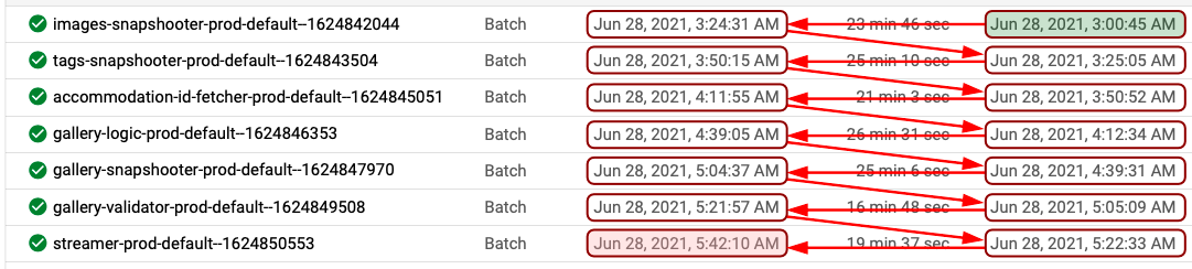
The next option was to create a simple orchestration framework to trigger the Dataflow jobs depending on the one just finished. We created a Cloud Log Sink to listen to the Dataflow job messages to detect the end of a job, then trigger a Cloud Function through a Pub/Sub topic with an event message, and trigger the next Dataflow job depending on which job has just completed.

We can have a simple workflow as shown below and trigger the next job with a little bit of programming.

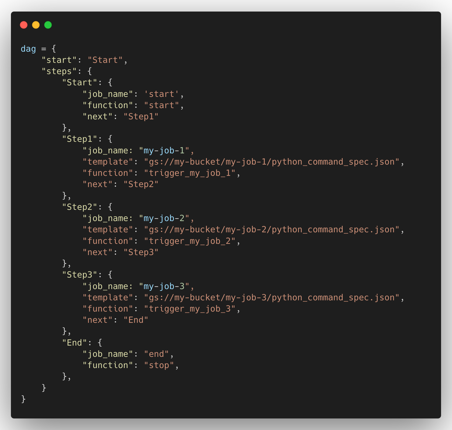
Even though this approach has some limitations such as not being able to have parallel executions of different Dataflow jobs, this is a completely serverless solution and has been working well for us over the last couple of months.

You can read more about the implementation details from this blog post.

Change Data Capture (CDC) Generation

Each gallery for a given accommodation can consist of hundreds of images, each having an image URL and a field for the sorting order: the position of the corresponding image in the image gallery. Even though we have to recalculate the entire image gallery for an accommodation even when a single image changed, we shouldn’t stream everything to the frontend. We should only stream out the changes for a given image with its image URL and the position of the gallery in order to avoid redundant records in the Kafka stream.

Imagine we had to recalculate the image gallery for Hilton Hotel, Colombo (Sri Lanka) because one new image was added, leading to the gallery consisting of fifty images. Depending on the position in which this new image gets inserted into the new gallery, we can have from fifty updates (when the new image becomes number one) to only one update (when it becomes the last). In any of these scenarios, we should only stream out the changed records.

In order to do this, we should compare today’s galleries with the last snapshot. Depending on whether a given image is present on the previous snapshot and today’s gallery, we can determine what kind of record should be streamed.

For instance, for a given accommodation:

1. If the image is present in today’s gallery, but not in the previous snapshot, then it’s a new image and we should stream out the new record.
2. If the image is present in both today’s gallery and previous snapshot, then we decide to stream out only if the content of the record (i.e. sorting order) has changed.
3. If an image is present in the previous snapshot, but not in today’s calculated gallery, it means this image got deleted and we should stream out a delete record (value as null).

One potential edge case we should consider is the last scenario above. Because we do not calculate the galleries for the entire dataset, but only for those accommodations changed, we’ll generate galleries only for a small number of accommodations and then the last scenario can result in streaming out deletes for all the unchanged images. To avoid this, we check if a given accommodation is marked as changed (by Changed Accommodations Fetcher) and generate a delete only if it was changed.

Snapshotting

Let’s say an advertiser (i.e. Expedia) gives us a new image for a hotel. This can cause us to recalculate the entire image gallery for that particular hotel depending on the contents and the quality of the image. And we shouldn’t recalculate the gallery multiple times if we get multiple changes for a given accommodation. To tackle this problem, we’re using snapshots to represent the entire dataset at a given moment. This helps us to extract all the images for a given accommodation when one or more images have changed.

Here is how we generate our snapshots.

Snapshot(Dn): Snapshot(Dm) + Changes(Dm to Dn)

Let’s say our pipeline started 1st of June 2021, and it’s been running since then. When the pipeline ran on the 1st of June, snapshot for that day will only contain the CDCs of 1st of June as there was no previous snapshot to work with. The next snapshot can be calculated by applying the CDC from the 2nd of June on top of the snapshot from the 1st of June.

If today is 1st of July, we can generate the snapshot for today by applying today’s CDC on top of the snapshot from yesterday: 30th of June. If our snapshooter hasn’t run after the first time (on 1st of June) and we need to run it today (1st of July), we can generate today’s snapshot by applying all the CDCs from 2nd of June till today on top of the snapshot from 1st of June. Even if our entire pipeline hasn’t run after the 1st of June, we still can generate today’s snapshot by applying today’s CDC on top of the snapshot from the 1st of June. The important fact to remember is that we have to read the CDCs from the Accommodation Images and Image Tags from the corresponding days to generate today’s Gallery CDC.

We’re sinking our input (i.e. Images and Tags) using Kafka streams and they keep on writing files to our Data Lake: a common data storage shared across teams to data transferring, throughout the day. To avoid having partial processing of files, we always skip files written today and pick files until the day before.

On the contrary, when we generate the Image Gallery snapshot, we should include today’s changes in the last snapshot excluding the changes on that day. This means when we generate a snapshot we should include the changes from the starting day or the end day, but not both nor neither. Then all the snapshots will align properly just like a jigsaw puzzle.

The issue with grouping records

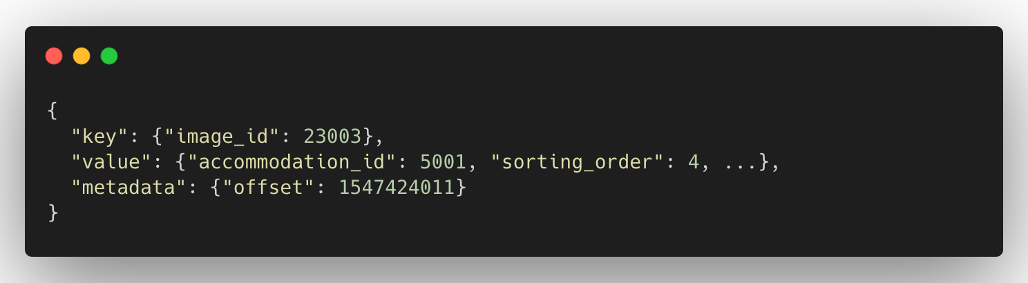
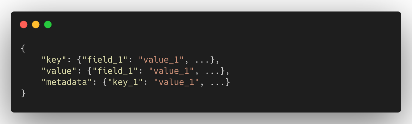
Now we have three snapshotting components in our pipeline creating snapshots of different datasets with different keys, and we didn’t want to have three different source codes for them. So we thought of having a shared code and parameterizing the behavior. All the records we consume and produce have the below-mentioned JSON format.

NOTE: CDCs will have null for the value field to denote delete statements, and those records are not present in the snapshots as they represent the final state of the dataset. However, different entities have different key fields, and also different fields for value and metadata.

One of the biggest issues we faced was grouping records for a given entity with the key. This transformation is required to pick the latest record for a given key in order to generate the snapshot. At first, we directly used the key object inside the record to generate the snapshot, but that approach has an issue.

Imagine we have two records with the same key, but the order of the fields is different.

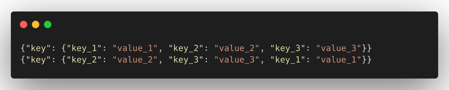
Even though these two records seem to be unique since they have the same composite key, Apache Beam considers these two records to have different keys because the order of the keys is different. Our deduction was that Apache Beam converts the keys into its own hashing format and it is dependent on the order of the fields. Since we don’t have control over the order of the fields written (by the previous Dataflow job), we had to generate a string key out of the key object in the record.

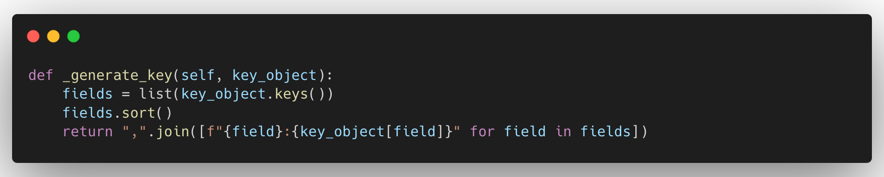
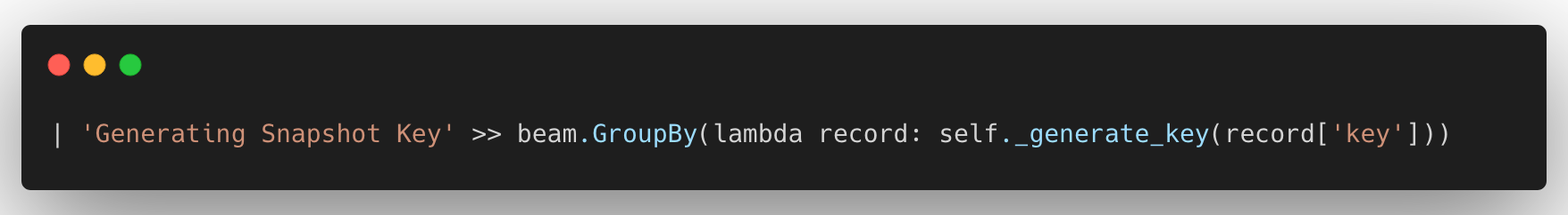
This ensures beam.GroupByKey() will properly group records with the same key despite the order of the fields.

Validation

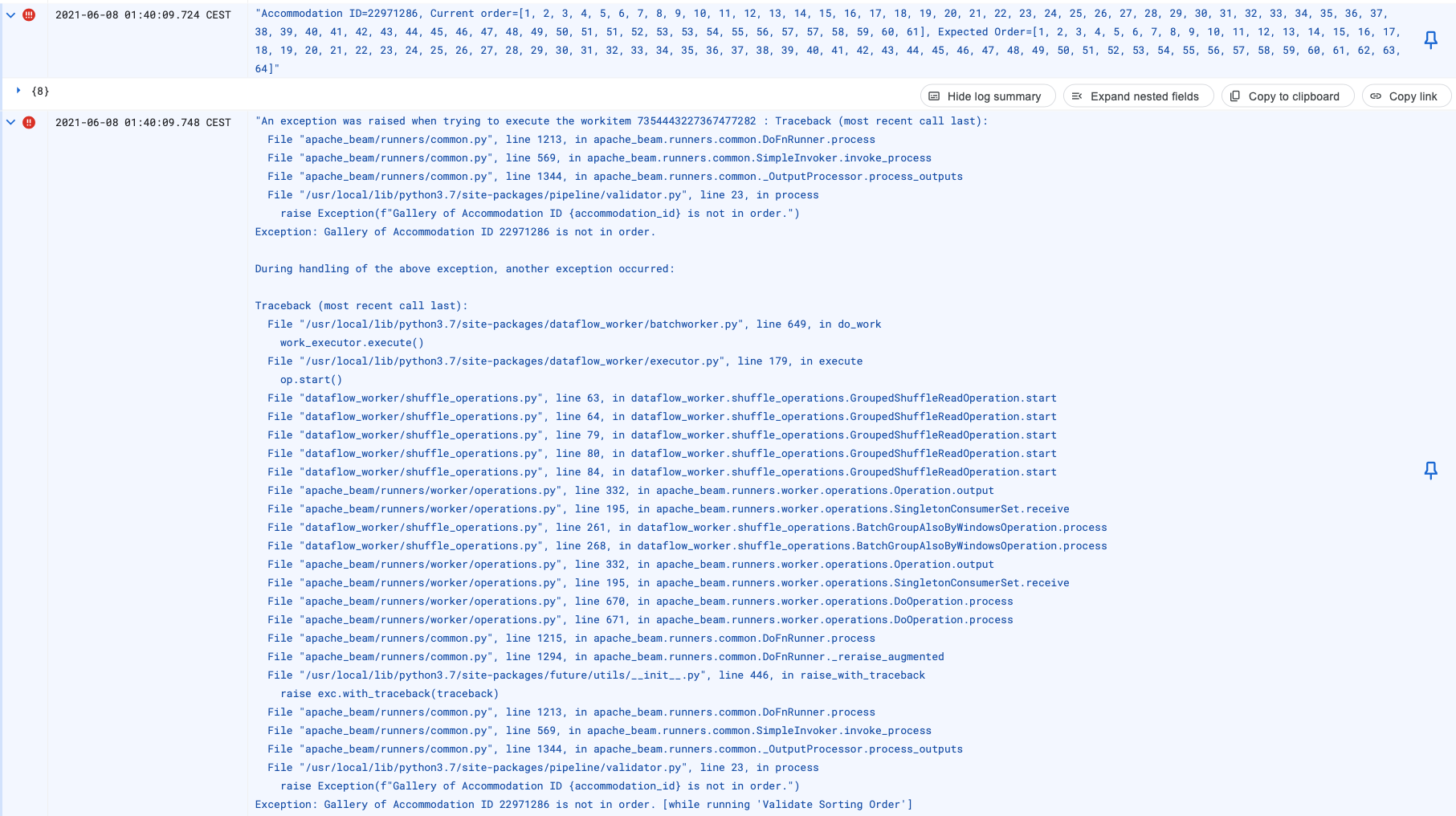
Regardless of how many unit tests and integration tests we have, we should still make sure that we’re not streaming out invalid galleries. One of the most important checks we should perform is to see if the images are in a continuous sequence. For instance, if a given accommodation has fifty images, the sorting order should be from one to fifty. This very simple, yet very powerful validation check has helped us to detect a lot of bugs in our pipeline and to prevent the frontend from showing corrupted galleries.

We also added two more validation rules to detect any corruptions in the daily snapshot. The Validator component checks if we have any delete records (where the value field is null) and all the non-delete records (updates and inserts) are present in the daily changes in the snapshot.

Streaming

Since the Streamer component is an Apache Beam pipeline, we can implement this using several user defined functions (also known as DoFns). Each DoFn can process multiple bundles of elements and each element is passed to the process method and we can perform our desired transformations there. We should consider batching these records in order to improve the performance of our component. However, we can’t detect the end of the entire dataset inside the process function. For instance, if we have 60 records to stream and we perform our DoFN on each record, we will trigger the process function 60 times.

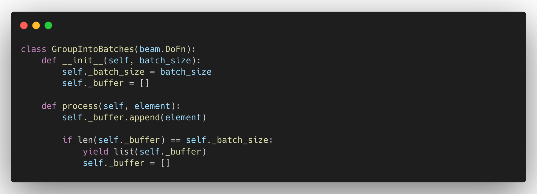
If we need to create batches of 25 records, it should create three batches with 25, 25, and 10 records. But the issue is that we wouldn’t know when to stream out the last 10 records because the process function is triggered per element/record and the last 10 records won’t fill the batch size. So if we only use the above approach, we will lose records.

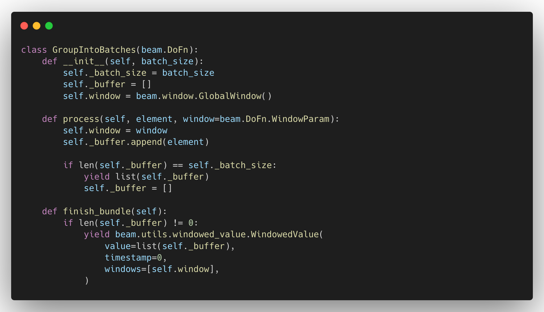
DoFNs have several methods we can override in order to perform initialization and clean-up tasks. The lifecycle of a DoFn is as follows [1].

• Setup - once per DoFn
• for each bundle
  • Start Bundle - once per bundle
  • Process - once per element
  • Finish Bundle - once per bundle
• Teardown - once per DoFn

For our use case, we either use teardown() or finish_bundle() methods to finish processing the remaining elements. However, Apache Beam discourages performing actions that are dependent on the input inside the teardown method, so we should use the finish_bundle() method here.

If we’re working with some resources such as database connections that we should initialize once and destroy at the end, we can use the Setup and Teardown methods.

Protobuf to JSON sink

We use Kafka topics heavily in trivago, to transfer data between teams, as well as cloud and data centers. Almost all of our Kafka topics have messages which are encoded with Protobuf to improve performance. Even though we usually sink them into a database, we recently started sinking these topics into GCS buckets in our DataLake as JSONL files.

Therefore we implemented a simple Python script using Google’s Proto to JSON mapper to sink our Kafka messages into a GCS bucket as JSONs. However, one of our Protobuf definitions had been using sfixed64 data type for some fields and they were sinking properly into databases as integers. However, when we wanted to sink them as JSON, protobuf library was sinking these fields as strings. We later found out the Protobuf to JSON converter provided by Google converts sfixed64 into strings [2]. Therefore, we use an explicit type conversion from sfixed64 into integers in our Dataflow jobs to avoid additional complications.

QAing the pipeline

Just like any pipeline or any software product, we should do a proper QA for our new pipeline to make sure we have galleries in the way we intended. As mentioned in the beginning, we had this pipeline in AWS which was implemented around AWS Glue, and we could use its output as the baseline to verify the output of the new pipeline we built on GCP.

We use Athena on top of Simple Storage Service (S3) and BigQuery on top of Google Cloud Storage (GCS) to analyze our data on AWS and GCP respectively. Since these two datasets live in two different cloud platforms, there is no straightforward way to compare them. We use Athena on top of Simple Storage Service (S3) and BigQuery on top of Google Cloud Storage (GCS) to analyze our data on AWS and GCP respectively. Since these two datasets live in different cloud platforms, there is no straightforward way to compare them.

So we decided to compare the two Kafka streams to check if the new output is the same as the one from the AWS pipeline. Even though this sounds simple, we had to compare more than 100 million images and more than a billion when you consider the number of records in the Kafka stream.

We could sink these Kafka streams to either AWS or GCP and perform a query, but we decided to go with the Hadoop cluster in our data center because of the convenience. We also considered the Storage Transfer Service by GCP to bring the files inside S3 buckets to GCS buckets and then perform BigQuery queries for the comparison. However, the files in S3 were in Parquet format and we didn’t want to spend more effort into converting them into JSONL or any other compatible file formats.

So we created two Hadoop Workflows to sink mirrors of the Kafka streams and executed a query to see how many images had different sorting_order compared to the AWS output. These Hadoop-Kafka sinks generate a Snapshot into a table and it saves the trouble of doing it ourselves within the query.

After the initial QA, we found out several bugs and decided to do the QA in GCP using BigQuery. We started sinking Kafka topics to GCS and created BigQuery tables on top of them so we can run our comparison queries.

The query we used is something similar to the below one.

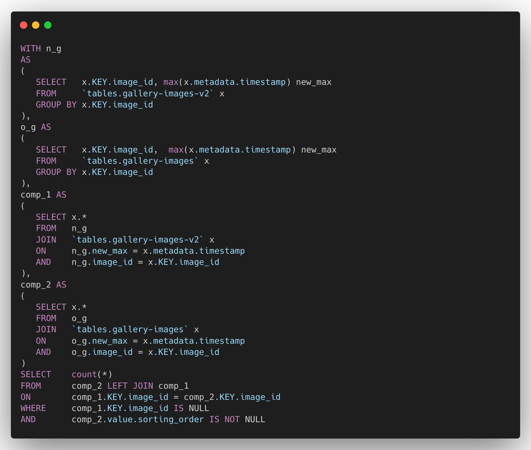
We also noticed BigQuery performs well in running these queries compared to AWS Athena and Hadoop, which significantly improved the QA process.

Summary

Developing an ETL pipeline for Cloud is not always easy, especially when we have multiple components handling millions of records and we have to properly orchestrate them. While migrating our Image Gallery pipeline from AWS to GCP, we faced a lot of challenges because we couldn’t do a lift-and-shift and had to re-design the pipeline entirely. However, this is still the first iteration of the migration for this pipeline and we’ll have more to finetune, to make it more flexible and performant.

References

[1] apache_beam.transforms.core module — Apache Beam documentation
[2] Language Guide (proto3) | Protocol Buffers